Real Income Tax Analysis

Introduction, Definitions, and Caveats #

It’s tax season, so what better way to celebrate than with a blog post about taxes. This post will be an analysis about inflation, income tax brackets, and their effects on real income over time.

This page gives a definition about tax bracket creep. In short, quoting from the article, “bracket creep occurs when inflation … pushes taxpayers into higher income tax brackets.”

We will be using Python and several libraries for our analysis:

• pandas
• NumPy
• Matplotlib

There are some things to keep in mind about the analysis:

• Excludes FICA (Medicare and Social Security) and state taxes
• Excludes above-the-line deductions
• Excludes credits like the AOTC and EITC
• Excludes additional standard deductions for those 65 and older and/or legally blind
• Excludes personal exemptions
• Does not take into account hidden taxes like those in the Omnibus Budget Reconciliation Act of 1990

As a result, this is a simplified model that does not account for the many complexities of tax. I wanted to get something published, but hope to address these shortcomings over time.

Gathering and Loading Data #

We’ll be working with CSV files from various sources:

• Tax Bracket Data
• Standard Deduction
• CPI Data

Now let’s begin with the code:

import pandas as pd
import matplotlib.pyplot as plt
import numpy as np

The above imports all the libraries we will be using.

tax_df = pd.read_csv("data/tax_brackets-1862-2025.csv")
standard_deduction_df = pd.read_csv("data/standard_deductions-1970-2025.csv")
cpi_df = pd.read_csv("data/CPIAUCSL-1947-2025.csv")

We use pd.read_csv() to read our CSV files into pandas DataFrames.

Cleaning Data #

The CSV files we are using need to be cleaned up. We will clean these DataFrames in order of difficulty, starting with standard deductions and ending with tax brackets/rates.

standard_deduction_df = standard_deduction_df.astype({"Year": str}).rename(
  columns={"Single": "Single Filer", "Married": "MFJ"}
)

The only changes we make are converting the year to a string for type uniformity and renaming the columns to match the columns of the other data frames.

cpi_df["observation_date"] = pd.to_datetime(
  cpi_df["observation_date"]
)  # convert from str to datetime to allow for datetime operations

cpi_df["year"] = cpi_df["observation_date"].dt.year  # extract the year from the date

updated_cpi_df = cpi_df.groupby("year")["CPIAUCSL"].mean()

modified_cpi_df = updated_cpi_df / updated_cpi_df.loc[2025]

Since the CPI is shown for each month, we calculate the annual CPI by averaging all the values for each calendar year. To do that, we convert the year from the type string to datetime to gain access to datetime functions that allow us to extract parts of the date. We extract the year from the date and group the years together. By grouping the years together, we can calculate the average CPI for each by simply running mean(). Finally, we recompute the values by setting the base year to 2025 to simplify later calculations.

The last part of this section is much more involved than the previous two:

redundant_columns = ["Unnamed: 2", "Unnamed: 5", "Unnamed: 8", "Unnamed: 11"]

rename_map = {
  "Married Filing Jointly (Rates/Brackets)": "MFJ Rates",
  "Unnamed: 3": "MFJ Brackets",
  "Married Filing Separately (Rates/Brackets)": "MFS Rates",
  "Unnamed: 6": "MFS Brackets",
  "Single Filer (Rates/Brackets)": "Single Filer Rates",
  "Unnamed: 9": "Single Filer Brackets",
  "Head of Household (Rates/Brackets)": "HoH Rates",
  "Unnamed: 12": "HoH Brackets",
}

updated_tax_df = (
  tax_df.dropna(how="all")  # remove empty rows
  .drop(columns=redundant_columns)  # remove rows with just '>' sign
  .rename(columns=rename_map)  # rename the columns
).reset_index(drop=True)  # hide the index

updated_tax_df

This code removes rows with NaN values, removes all columns containing ’>’ signs, and renames the columns to more appropriate names. You can take a look at the Marimo link above to see how the original CSV file was formatted.

rates_melted = updated_tax_df.melt(
  id_vars=["Year"],
  value_vars=["MFJ Rates", "MFS Rates", "Single Filer Rates", "HoH Rates"],
  var_name="Filing Status",
  value_name="Tax Rate"
)

brackets_melted = updated_tax_df.melt(
  id_vars=["Year"],
  value_vars=["MFJ Brackets", "MFS Brackets", "Single Filer Brackets", "HoH Brackets"],
  var_name="Filing Status",
  value_name="Income Bracket",
)

df.melt() basically unpivots, or changes the format from more columns and fewer rows to one with fewer columns and more rows. Doing this allows us to filter by “Year” and “Filing Status.” Again, you can look the Marimo link to see how the transformation works.

# Clean the names so they match
rates_melted["Filing Status"] = rates_melted["Filing Status"].str.replace(" Rates", "")
brackets_melted["Filing Status"] = brackets_melted["Filing Status"].str.replace(" Brackets", "")

# Join them together
final_tax_df = rates_melted.copy()
final_tax_df["Income Bracket"] = brackets_melted["Income Bracket"]

final_tax_df = final_tax_df.dropna().reset_index(drop=True)  # remove all NaN values

This takes the two melted tables and combines them into a single table. It first creates a copy of one of the DataFrames and then appends the relevant column to it. After that, we remove all NaN values.

final_tax_df["Tax Rate"] = final_tax_df["Tax Rate"].str.rstrip("%")

final_tax_df["Income Bracket"] = (
  final_tax_df["Income Bracket"]
      .str.lstrip("$")
      .str.replace(",", "")
)

We use the strip() variants and replace() remove extra characters and enable us to late easily transform these values into numeric types.

Putting Everything Together #

def calculate_standard_deduction(year, filing_status, income):
  # Calculate the standard deduction for years 1944 to 1969 (10% of AGI)
  if int(year) <= 1969:
      return min(1000, income * .10)
  else: 
      # Get the standard deductions for each filing status for that year
      standard_deduction = standard_deduction_df.loc[standard_deduction_df["Year"] == year]

      # Select column with the matching filing status
      standard_deduction = standard_deduction.loc[:, filing_status].iat[0].astype(int)

      return standard_deduction

This function calculates the standard deduction. From 1944 to 1969, the standard deduction was based on the gross adjusted income, up to a maximum of $1000. From 1970 onwards, we use the provided standard deduction amounts. We use iat to get the value independent of the data frame. loc allows you to filter values against both rows and columns with the format .loc[rows, columns].

def calculate_tax_liability(year, filing_status, income):
  # Get the brackets and rates for the year and filing status
  tax_info = final_tax_df[
      (final_tax_df["Year"] == year) & (final_tax_df["Filing Status"] == filing_status)
  ].astype({"Tax Rate": float, "Income Bracket": int})

  # Because of the offset, we will use a different method to calculate the tax brackets

  # total income taxed at 10%
  # (total income - 11,925) taxed at (12-10)%

  tax_info["Updated Tax Rate"] = np.diff(tax_info["Tax Rate"], prepend=0)
  tax_info

  # Calculate the amount owed for each bracket
  tax_liability_brackets = np.maximum(income - tax_info["Income Bracket"], 0) * (
      tax_info["Updated Tax Rate"] / 100
  )

  return np.sum(tax_liability_brackets)

This function calculates the tax liability. We first convert the tax rate and income bracket into numeric types to allow for calculations. If done manually, we would calculate the amount owed by adding the income for a bracket. For example, if we have a single filer for 2025 with $60,000 taxable income:

$60000 - 48475 \Rightarrow 11525 * .22 = 2535.50$

$48475 - 11925 \Rightarrow 36550 * .12 = 4386$

$11925 - 0 \Rightarrow 11925 * .10 = 1192.50$

Adding these all up, we get $8114$.

However, I decided to use the difference between the rates for each bracket instead. The first bracket would remain 10%, while the second and third would become 2% (12-10) and 10% (22-12), respectively. Using the same scenario:

$60000 - 0 \Rightarrow 60000 * .10 = 6000$

$60000 - 11925 \Rightarrow 48075 * .02 = 961.50$

$60000 - 48475 \Rightarrow 11525 * .10 = 1152.5$

Here, we also get a sum of $8114$.

# The function takes in year, filing status, income and spits out the real income

def calculate_real_income(year, filing_status, income):
  standard_deduction = calculate_standard_deduction(year, filing_status, income)
  taxable_income = income - standard_deduction

  tax_liability = calculate_tax_liability(year, filing_status, taxable_income)
  after_tax_income = income - tax_liability

  return after_tax_income / modified_cpi_df.loc[int(year)]

This function returns the real income based on year, filing status, and income. It uses the two functions we created above. We divide the after-tax income by the CPI index to adjust for CPI changes. The steps for calculating the real income are as follows:

• Taxable Income = Gross Income - Standard Deduction
• (Nominal) After-Tax Income = Gross Income - Tax Liability
• Real After-Tax Income = Nominal After-Tax Income / CPI Adjustment

Graphing the Data #

years = range(year_min, year_max + 1)

data = []
for y in years:
  nominal_needed = income * modified_cpi_df.loc[y]

  real_income = calculate_real_income(str(y), filing_status, nominal_needed)
  data.append({"Year": y, "Real Income": real_income})

comparison_df = pd.DataFrame(data)

comparison_df

Since we want the results across a range of years, we gather all the results into a list and convert that list into a DataFrame for graphing. We also need to adjust the gross income by the CPI.

comparison_df.set_index("Year").plot(
  kind="line",
  figsize=(12, 8),
  grid=True,
  title="Real Income Adjusted for Inflation (1947–2025)",
  ylabel="2025 Real Dollars ($)"
)

We set the index to “Year” to display it as the x-axis. We also add an appropriate title and label for the y-axis.

Conclusion #

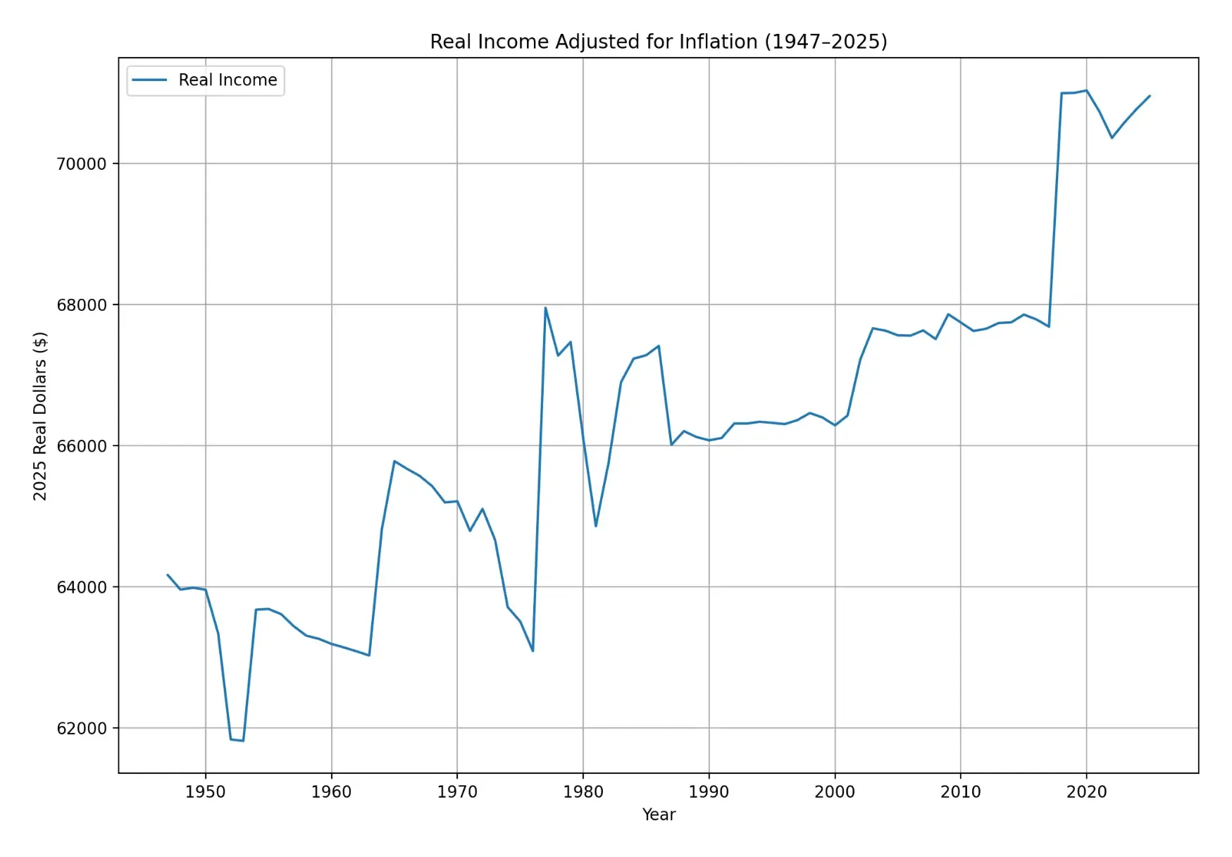
As we see from the graph, there hasn’t been any bracket creep recently at the federal level. In fact, real income has been increasing as a result of legislation.

Bonus: Here’s an interesting article about tax regulations and their obscure effects on society